Chapter 2 Introduction to R
This unit spans Mon Feb 03 through Sat Feb 08.
At 11:59 PM on Sat Feb 08 the following items are due:
- DC 4 - Introduction to R: Factors
- DC 5 - Introduction to R: Data frames
- DC 6 - Introduction to R: Lists
Unit 2 further builts on unit 1 and introduce you to remaining building blocks in R. It is a chance for you to breathe, assimilate what you have already learned and review whatever you think needs additional focus. We will start building up the pace again through unit 5. At that point, things should start to smooth out a bit. We’ll have covered enough R to take in a data set, clean it, and present it visually.
2.1 Media
- Reading: R-FAQ 2.10 - What is CRAN?
- Reading: R Packages: A Beginner’s Guide
- Video: Introduction to R
2.2 Lists
A list is a generic vector that doesn’t need to contain the same primitive data types. This makes referencing members a little more complex. We use the list function to create lists. Like matrices, we won’t be using lists much in this class so I’ll provide just a brief introduction.
num <- c(1,2,3)
names <-  c("Fred", "Ethel")
status <- c(TRUE, TRUE, FALSE, FALSE)
l <- list(num, names, status, 5)
l[2]
## [[1]]
## [1] "Fred" "Ethel"## [1] "Ethel"Lists can get pretty tricky but notice if we use a single bracket, the object returned is another list so l[2] returns a list of one which contains a character vector with two elements. Using the double-bracket returns the actual element so l[[2]] returns a character vector of two elements. This is why when we type l[[2]][2] we are saying return the second element of the character vector (i.e., Ethel) whereas if we typed l[2][2] we would get an out of bounds because the list returned with l[2] contains only one element. l[2][[1]][2] would return a list of one, then take the first item in that list (a character vector) and return the second item in that vector – which would be identical to typing l[[2]][2]. While we won’t be working much with lists directly this semester, it is helpful to go back and review them at a later date because we will be using a specialized form of a list throughout the semester, namely – the data frame.
2.2.1 Data Frames
Data frames are lists that we can metaphorically think of as spreadsheets with some restrictions:
- variable names (i.e., column names) must be unique within the data frame
- all elements (columns) in the data frame are vectors.
- all elements (columns) in the data frame have equal length.
So when your data is in a format where columns represent variables, and rows typically represent an observation, data frames are the object that you most likely want to use to represent this data. Most forms of structured data fit nicely into a data frame.
We use the data.frame function to create a data frame.
rooms <- c("Living Room", "dining room", "kitchen")
colors <- c("Navaho White", "Stonington Gray", "Edgecomb Gray")
comments <- c("Patch ceiling hole - Bob", "Use a tinted primer - Joe",
             "Look's pretty good - Ann")
price <- c(245.30, 300, 180.25)
house <- data.frame(rooms, colors, comments, price, stringsAsFactors = FALSE)
We created a data frame from the vectors we worked with earlier. They are all equal length and have the same data within the vectors. We can also view the data by clicking on the table icon next to the house variable in the environment pane and see the table as shown below.
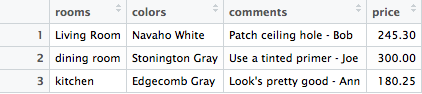
dataframe
Each column can be referenced by the convention variable_name$column_name, for example, house$price will return the price column as a numeric vector. I can also interact with it as we did with mtcars in the last lesson. I can reference rows and columns in a few different ways.
- by index - e.g.,
house[1,2]will return the first row, second column of the data frame - by name - e.g.,
house[1, "colors"]will return the first row of thecolorscolumn - by name - e.g.,
house$colorswill return thecolorscolumn as a character vector as willhouse[,"colors"] - by list index - e.g.,
house[2]will return the second column as a data.frame object as willhouse["colors"] - by list index - e.g.,
house[[2]]will return the second column as a character vector as willhouse[,2]
You can also select multiple rows and columns by using combine and/or ranges (e.g., house[1:2, c("rooms", "colors")])
Finally, you can search for specific values in a data frame as shown below.
##         rooms       colors                 comments price
## 1 Living Room Navaho White Patch ceiling hole - Bob 245.3## rooms colors comments price
## 1 Living Room Navaho White Patch ceiling hole - Bob 245.3
## 2 dining room Stonington Gray Use a tinted primer - Joe 300.0Once again, you can see that there are many different ways to accomplish the same task in R. Everything that we’ve done so far has been using the base packages in R (i.e., the stuff installed by default). In the next unit, we’ll show how to search within a data frame using additional packages that aren’t installed by default. We’ll also explain packages, the concept of tidy data, and go into more depth with data frames.
2.3 Factors
When you first took statistics, you learned about different types or classification of variables. One reason why variable types become essential is that they determine the kind of analysis that can be performed. Generally speaking, we can classify data as being numeric (e.g., height, weight, salary), categorical (e.g., gender, color, hometown), or ordinal. Right now, we are not concerned with the numeric data.
Let’s start off by creating some data of houses we might have looked at when thinking about purchasing a property
description <- c("blue cape near university", "small bungalo near ocean",
                "weird oval shaped home", "shag carpet place that smells like beer",
                "block shaped home on busy street")
price <- c(250000, 400000, 185000, 172000, 180000)
color <- c("blue", "blue", "yellow", "yellow", "green")
initial_impressions <- c("love", "love", "hate", "neutral", "hate")
houses <- data.frame(description, price, color, initial_impressions, stringsAsFactors = FALSE)
summary(houses)
## description price color initial_impressions
## Length:5 Min. :172000 Length:5 Length:5
## Class :character 1st Qu.:180000 Class :character Class :character
## Mode :character Median :185000 Mode :character Mode :character
## Mean :237400
## 3rd Qu.:250000
## Max. :400000Looking at a summary of the houses data, I see some detailed statistics regarding price but the other summary information is relatively meaningless. Let’s make a minor modification to our data frame.
##  description            price           color   initial_impressions
##  Length:5           Min.   :172000   blue  :2   Length:5
##  Class :character   1st Qu.:180000   green :1   Class :character
##  Mode  :character   Median :185000   yellow:2   Mode  :character
##                     Mean   :237400
##                     3rd Qu.:250000
##                     Max.   :400000
Notice that the summary for color now includes a count of the different colors. This is because we instructed R to make color a factor. Also notice when I created the data frame, I used the parameter stringsAsFactors = FALSE to tell R not to create factor variables from character data, which is the default behavior.
## 'data.frame':    5 obs. of  4 variables:
##  $ description        : chr  "blue cape near university" "small bungalo near ocean" "weird oval shaped home" "shag carpet place that smells like beer" ...
##  $ price              : num  250000 400000 185000 172000 180000
##  $ color              : Factor w/ 3 levels "blue","green",..: 1 1 3 3 2
##  $ initial_impressions: chr  "love" "love" "hate" "neutral" ...
Looking at the structure of color we can see that it is now defined as a factor with three levels (blue, green, and yellow). Internally, factors get stored as integers, but we now need to be careful when we treat them as strings. By default, a factor has levels that are in alphabetical order that corresponds to the integer values. In this case:
- 1 = blue
- 2 = green
- 3 = yellow
Now we can go back and follow the same process to make initial_impressions a factor.
##  description            price           color   initial_impressions
##  Length:5           Min.   :172000   blue  :2   hate   :2
##  Class :character   1st Qu.:180000   green :1   love   :2
##  Mode  :character   Median :185000   yellow:2   neutral:1
##                     Mean   :237400
##                     3rd Qu.:250000
##                     Max.   :400000
You’ll notice that the levels of initial_impressions, like color are also in alphabetical order. In reality, hate < neutral < love, which suggests that this might be an ordinal variable and not a categorical variable. If we want to have a worst-to-first type of order, we can specify this when creating the factor by setting the parameters levels and ordered.
houses$initial_impressions <- factor(houses$initial_impressions, levels = c("hate", "neutral", "love"), ordered = TRUE)
summary(houses)
## description price color initial_impressions
## Length:5 Min. :172000 blue :2 hate :2
## Class :character 1st Qu.:180000 green :1 neutral:1
## Mode :character Median :185000 yellow:2 love :2
## Mean :237400
## 3rd Qu.:250000
## Max. :400000We have told R to make initial_impressions an ordered factor.
## 'data.frame':    5 obs. of  4 variables:
##  $ description        : chr  "blue cape near university" "small bungalo near ocean" "weird oval shaped home" "shag carpet place that smells like beer" ...
##  $ price              : num  250000 400000 185000 172000 180000
##  $ color              : Factor w/ 3 levels "blue","green",..: 1 1 3 3 2
##  $ initial_impressions: Ord.factor w/ 3 levels "hate"<"neutral"<..: 3 3 1 2 1
If you have to clean and transform your data, it is often advisable not to use factors until right before you analyze data. This will become more apparent later in the semester. We’ll also show you a different way to order factors using the forcats package in a few units.
2.4 Tibbles
Finally, I want to briefly introduce you to an updated version of the data frame – the tibble. It isn’t going to make much sense yet, but tibbles make data frames slightly less frustrating to work with. For a full explanation, see the package definition, but it will become more evident after you have had more exposure to R. One thing you might notice is that they print a little more nicely. We won’t be interacting with tibbles too much, but they will pop up again during the semester.
##                               description  price  color initial_impressions
## 1               blue cape near university 250000   blue                love
## 2                small bungalo near ocean 400000   blue                love
## 3                  weird oval shaped home 185000 yellow                hate
## 4 shag carpet place that smells like beer 172000 yellow             neutral
## 5 block shaped home on busy street 180000 green hate## # A tibble: 5 x 4
## description price color initial_impressions
## <chr> <dbl> <fct> <ord>
## 1 blue cape near university 250000 blue love
## 2 small bungalo near ocean 400000 blue love
## 3 weird oval shaped home 185000 yellow hate
## 4 shag carpet place that smells like beer 172000 yellow neutral
## 5 block shaped home on busy street 180000 green hate2.5 Packages
Packages are a collection of functions and data sets that are typically not a part of base R (i.e., they are developed by the community). While functions like mean, median, max, etc. are part of base R, the as_tibble function we just used is part of the tibble package which is loaded with dplyr.
To install a package, we can use the install.packages() command or we can select Tools –> Install Packages in RStudio. By default, the available packages listed are from the CRAN repository, but we can also install packages from Bioconductor or Github.
After a package is installed, if we want to use the functions or data sets that come with the package, we must load it using the library function as we have already done with dplyr and knitr.
Some R packages have overviews of the package, called a “vignette”. You can see what vignettes are available for packages that you have loaded using the browseVignettes function. This will launch a browser tab with links to the vignettes. You can also find out what packages and versions you have loaded, along with other useful information, by using the sessionInfo function as shown below. There will probably be more loaded than you expect as many packages have dependencies (i.e., they load other packages). We’ll probably be using sessionInfo to diagnose some problems students might have during the semester.
## R version 3.6.2 (2019-12-12)
## Platform: x86_64-apple-darwin15.6.0 (64-bit)
## Running under: macOS Catalina 10.15.4
##
## Matrix products: default
## BLAS:   /Library/Frameworks/R.framework/Versions/3.6/Resources/lib/libRblas.0.dylib
## LAPACK: /Library/Frameworks/R.framework/Versions/3.6/Resources/lib/libRlapack.dylib
##
## locale:
## [1] en_US.UTF-8/en_US.UTF-8/en_US.UTF-8/C/en_US.UTF-8/en_US.UTF-8
##
## attached base packages:
## [1] stats     graphics  grDevices utils     datasets  methods   base
##
## other attached packages:
## [1] dplyr_0.8.4 knitr_1.26
##
## loaded via a namespace (and not attached):
##  [1] Rcpp_1.0.4       rstudioapi_0.11  magrittr_1.5     tidyselect_0.2.5
##  [5] R6_2.4.1         rlang_0.4.5      fansi_0.4.1      stringr_1.4.0
##  [9] highr_0.8        tools_3.6.2      xfun_0.11        png_0.1-7
## [13] utf8_1.1.4       cli_2.0.2        htmltools_0.4.0  yaml_2.2.0
## [17] digest_0.6.25    assertthat_0.2.1 tibble_2.1.3     crayon_1.3.4
## [21] bookdown_0.16.5  purrr_0.3.3      vctrs_0.2.4      glue_1.3.2
## [25] evaluate_0.14    rmarkdown_2.0    stringi_1.4.6    compiler_3.6.2
## [29] pillar_1.4.3     pkgconfig_2.0.3
Most of the packages we will use in this course are part of the tidyverse, which we will introduce in the next unit.
2.6 DataCamp Exercises
This unit’s DataCamp exercises have you finishing their Introduction to R course, which gives you the prerequisite knowledge required for many of their other courses.