Chapter 6 Creating Reports

This unit spans Mon Mar 02 through Sat Mar 07.
At 11:59 PM on Sat Mar 07 the following items are due:

• DC 13 - Communicating with Data in the Tidyverse: Introduction to RMarkdown
  
• DC 14 - Communicating with Data in the Tidyverse: Customizing your RMarkdown report

The workload for this unit is slightly less than most, but we are preparing you to complete your first assignment in the next unit. We’ll cover formatting and publishing reports using R Markdown.

6.1 Media

• Markdown Tutorial, an interactive tutorial – start here.
• R Markdown Gallery, look at the “Documents” examples.
• R Markdown Cheatsheet, a good, quick reference.

6.2 R Markdown

Before we can explain R Markdown, we need to explain Markdown. Markdown is a straightforward markup language for formatting text that was developed by John Gruber in 2004. For example, if I enclose a word or phrase with underscores like this: _hello, I am italic_ it will render in italics as shown below.
hello, I am italic

Some other common markdown formats are shown below:

• **bold**
• `code`
• [hyperlinked text](url)
• ![optional caption text](path/to/img.png)
• # 1st level header
• ## 2nd level header
• * bullet item 1
• * bullet item 2
• …and others.

R Markdown uses an extended form of markdown known as Pandoc Markdown. If you want to see a list of the available Pandoc markdown codes, in RStudio, select Help --> Cheatsheets --> R Markdown Cheat Sheet and look at the left side of the second page.

R Markdown combines Pandoc Markdown formatting with the ability to display and run R code and show the output. R Markdown contains three essential components.

1. an optional YAML header, enclosed with ___
2. R code chunks, enclosed with ```
3. Text formatting using Pandoc Markdown.

In RStudio, select File --> New File --> R Markdown... and accept the default options and click OK. Take a look at the default contents of the new R Markdown file. Click Knit on the top of your editing window and notice that RStudio wants to name the document with a .Rmd extension. Go ahead and save the file and look at the knitted or rendered output. Notice the code, the output, and the visualization. Let’s take a look at some of the elements of the actual R Markdown file.

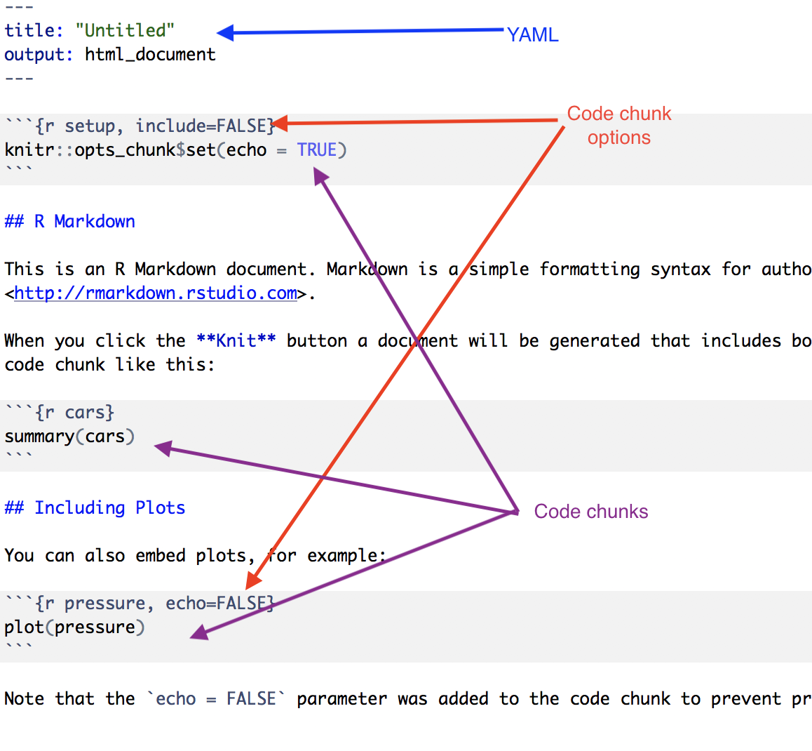
The front-matter or YAML portion of the document is being used to specify the title of the document – in this case, “Untitled”, and the output format – in this case, HTML. Note that this portion is delimited by three hyphens ---.

6.2.1 code chunks

The code chunks are delimited by three back-ticks ``` and, in this case, start with {r} which designates the language being used (we’ll only be using R in this course). The code in these sections runs and, by default, is displayed in the document and rendered to look different than regular text visually (i.e., it is usually in a grey box using a monospaced font).
The code chunk options are settings that we use to control the behavior of the code chunk. More common options include

• include = FALSE prevents code and results from appearing in the finished file. R Markdown still runs the code in the chunk, and other chunks can use the results.
• echo = FALSE prevents code, but not the results from appearing in the finished file. This is a useful way to embed figures.
• results = "hide" displays code and not output.
• message = FALSE prevents messages that are generated by code from appearing in the finished file.
• warning = FALSE prevents warnings that are generated by code from appearing in the finished.

The chunk name is optional, but it is good practice to name your chunks because it makes troubleshooting easier. If you want to look at some more chunk options, reference the R Markdown Reference Guide and see the knitr chunk options section (R Markdown uses the knitr library).

6.2.2 inline code

We can also write code inline in our report without a code chunk by enclosing the inline code using <backtick> r <code> <backtick>. For example, one plus four equals 5.

In the sentence above, I typed one plus four equals `r 1+4`.

6.3 YAML options

There are a variety of formatting options specific to HTML documents in r markdown that are controlled through YAML options. Many of the options start with the output: html_document in the front matter as shown below. I’ll use some of the more common options and explain.

---
title: "My document"
author: "Me"
output:
  html_document:
    toc: true
    toc_float: true
    number_sections: true
    code_folding: hide
---

In the example above:

• toc: true specifies a table of contents (clickable links pointing to level 1 headers)
• toc_float: true has the table of contents floating to the left of the document (much like this course website).
• number_sections: true start table of contents numbering at one and increasing by one.
• code_folding: hide allows you not to display code and have a clickable show code button if the reader wants to see the code.

There are many other options available, and you can read about them in the html_document_format publication by RStudio.

6.4 Embedding plots

To date, we haven’t really created visualizations in R. There are many packages that extend the base graphics available to us in R. We will be using the ggvis package for most of this semester – it will also be prominently used in the visualization course.

Embedding plots in R Markdown is pretty straightforward but there are a couple of things we need to consider:

1. What format is my final report going to be output to (e.g., html, pdf, Word, ioslides, etc.).
2. How are my reader’s going to consume my report (desktop/laptop, mobile device, printed)

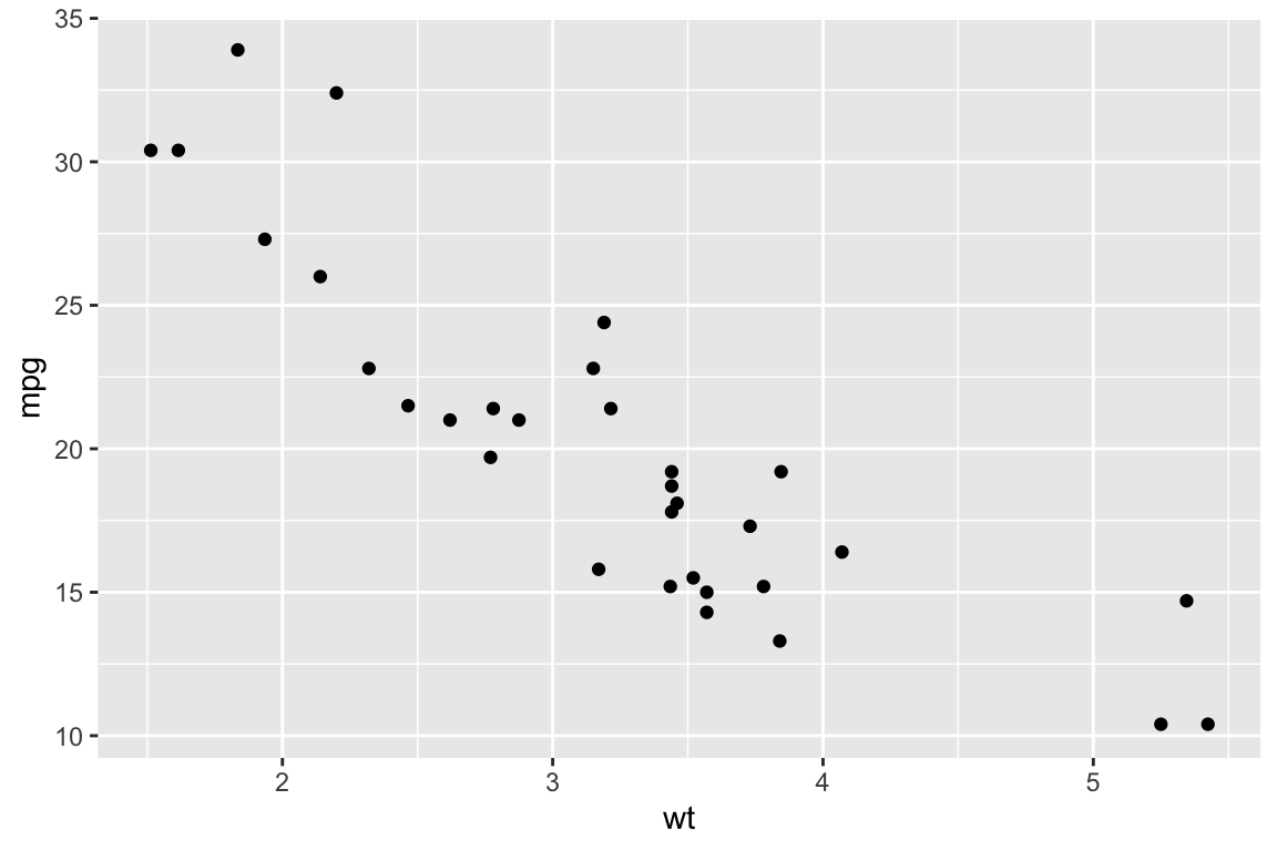
For this unit, we’ll just be working with html because it is the most dynamic form of output. For figures, we might want to set the fig.width and fig.height. If we don’t, they will default to seven (measurements are in inches). In the image below, I have fig.width=6 and fig.height=8.

library(tidyverse)
mtcars %>% ggplot(aes(wt, mpg)) + geom_point()

6.5 Prettier tables

There are some decent formatting options for tables in R Markdown. Below are three different versions of the same table:

Default

output <- head(mtcars %>% select(wt, mpg), 10)
output

##                      wt  mpg
## Mazda RX4         2.620 21.0
## Mazda RX4 Wag     2.875 21.0
## Datsun 710        2.320 22.8
## Hornet 4 Drive    3.215 21.4
## Hornet Sportabout 3.440 18.7
## Valiant           3.460 18.1
## Duster 360        3.570 14.3
## Merc 240D         3.190 24.4
## Merc 230          3.150 22.8
## Merc 280          3.440 19.2

kable

library(knitr)
kable(output, digits = 2)

	wt	mpg
Mazda RX4	2.62	21.0
Mazda RX4 Wag	2.88	21.0
Datsun 710	2.32	22.8
Hornet 4 Drive	3.21	21.4
Hornet Sportabout	3.44	18.7
Valiant	3.46	18.1
Duster 360	3.57	14.3
Merc 240D	3.19	24.4
Merc 230	3.15	22.8
Merc 280	3.44	19.2

pander

library(pander)
panderOptions('round', 2)
set.caption("mtcars weight and mpg")
pander(output)

mtcars weight and mpg

	wt	mpg
Mazda RX4	2.62	21
Mazda RX4 Wag	2.88	21
Datsun 710	2.32	22.8
Hornet 4 Drive	3.21	21.4
Hornet Sportabout	3.44	18.7
Valiant	3.46	18.1
Duster 360	3.57	14.3
Merc 240D	3.19	24.4
Merc 230	3.15	22.8
Merc 280	3.44	19.2

There are several other table formatting packages that we aren’t going to cover but to summarize:

• default tables aren’t too pretty
• kable is part of knitr and is a simple way to make prettier tables
• pander has more options than kable, but is more complex
• there are a variety of other packages that might suit your specific need (e.g., xtable, htmltables, etc.) but for this class pander and kable should have you covered.

6.6 Knitting

At any time, you can knit your R Markdown file. In RStudio, you can use the Knit or KnitHTML button to specify if you want to knit to html, pdf, or a Microsoft Word document. What actually happens behind the scenes is that RStudio uses the rmarkdown package to render the output in your specified format. The video will have more detailed use of R Markdown.

6.7 DataCamp Exercises

The two DataCamp chapters for this unit are all about working with R Markdown and will help develop your skills at creating beautiful reports. Keep in mind that many of the neat things that you can do rendering HTML are not available for pdf or MS Word documents.